HMM Part 1
Learning about Hidden Markov Modelling (HMM)
Who is Markov and what was he modeling?
Andrey Markov was a Russian mathemetician, who studied stochastic processes. His big contribution was Markov chains/processes. A Markov chain is a way of modeling a sequence of possible events, or states, where the probability of a future state is dependent upon the current state, and not on anything that happened before. So what does that mean?
Let's use the weather as an example, where we have three possible states: rain, snow, and sunshine. We can summarize the possible weather states in a graph, with the three states connected by arrows showing the probability of transitioning from one state to another.
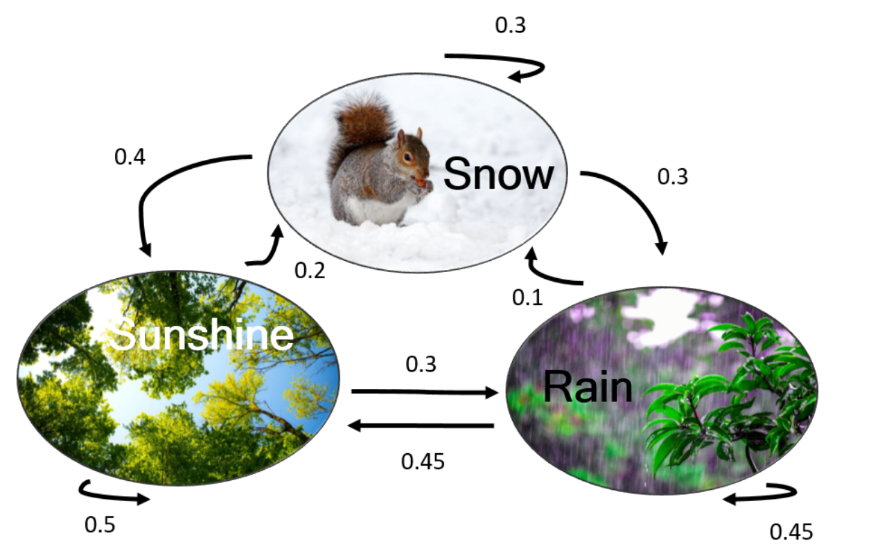
If we look at the transition probabilities between rain and sunshine, we see that if it was raining yesterday, there is a 45% chance that it will be sunny today. And if yesterday was sunny, there's a 30% chance that it will rain today.
The Markov chain can be described by a transition probability matrix, P:
$$ P = \begin{bmatrix} 0.3 & 0.3 & 0.4 \\ 0.1 & 0.45 & 0.45 \\ 0.2 & 0.3 & 0.5 \end{bmatrix} $$where the pre-transition states are the rows (snow, rain, sun), and the post-transition states are the columns (snow, rain, sun).
- Row 1: starting at snow
- Row 2: starting at rain
- Row 3: starting at sun
- Column 1: moving to snow
- Column 2: moving to rain
- Column 3: moving to sun
We can therefore use the matrix to determine the probability of moving from any state i to any other state j. So if we want to know the probability that it will be snowing tomorrow if it is snowing today, $$P_{i,j} = P_{1,1} = 0.3$$ and the probability that it will be sunny tomorrow if it is raining today is $$P_{i,j} = P_{2,3} = 0.45$$
In some cases, we are also given a vector of initial probabilities, which are the probabilities of being in any of the given states at time t=0. We might think of this as our best guess for the weather today. Since we're in California and it's spring time (or is it summer now? I've lost track), let's say we have a 0% chance of snow, a 20% chance of rain, and an 80% chance of sunshine today. We can represent these values in a similar notation as our transition matrix.
$$ \pi_0 = \begin{bmatrix}0 \\ 0.2 \\ 0.8 \end{bmatrix} $$Notice the order of the states in rows is the same as in the transition matrix, i.e. first snow, then rain, and finally sunshine.
At first it might seem a little complicated to bother with initial probabilities since don't we always know exactly we start? The short answer is yes if we're simulating a single sequence of weather states, but in general it's convenient to use initial probabilities to both incorporate uncertainty as well as to model the average behavior of the system over time. You can think of this example as equivalent to tracking 100 sequences simultaneously where 0, 20, and 80 of those simulations begin with snow, rain, and sun, respectively.
Now that these initial probabilities have given us a starting point, we can use our Markov chain to make predictions about future weather states. So let's say we have our matrix as defined above, and we know today's initial probabilities, and the transition probabilities for moving between each state. What is the probability that it will rain tomorrow? This at first seems like a complicated question since we have to account for the movements between all pairs of states. (What fraction of sunny days become rainy? What fraction of rainy days lead to snow?) Conveniently, there is a direct correspondence between the calculations we need to make and matrix multiplication, so we can answer this question by taking the product of our transition matrix and our initial probabilities.
$$ \pi_1 = \begin{bmatrix} 0.3 & 0.3 & 0.4 \\ 0.1 & 0.45 & 0.45 \\ 0.2 & 0.3 & 0.5 \end{bmatrix} \begin{bmatrix}0 \\ 0.2 \\ 0.8 \end{bmatrix} = \begin{bmatrix}0.38 \\ 0.45 \\ 0.45 \end{bmatrix} $$Our output is set of probabilities organized just like our initial one but with the numbers changed to reflect the evolution of our system over the course of one day. We can keep iterating like this to simulate an arbitrary number of days. For example, the probabilities for day 2 are:
$$ \pi_2 = \begin{bmatrix} 0.3 & 0.3 & 0.4 \\ 0.1 & 0.45 & 0.45 \\ 0.2 & 0.3 & 0.5 \end{bmatrix} \begin{bmatrix}0.38 \\ 0.45 \\ 0.46 \end{bmatrix} = \begin{bmatrix}0.433 \\ 0.4475 \\ 0.441 \end{bmatrix} $$This turns out to be the same as multiplying our initial probabilities by the square of the transition matrix and likewise with higher powers. We can use this to take a little shortcut if we want to know where our system will be further out in the future. Instead of repeating the above calculation over and over, we can instead directly powering up the matrix to the number of days we want to move forward. Thus, the probabilities for day 100 are given by:
$$ \pi_{100} = \begin{bmatrix} 0.3 & 0.3 & 0.4 \\ 0.1 & 0.45 & 0.45 \\ 0.2 & 0.3 & 0.5 \end{bmatrix}^{100} \begin{bmatrix}0 \\ 0.2 \\ 0.8 \end{bmatrix} = \begin{bmatrix}0.44183 \\ 0.44183 \\ 0.44183 \end{bmatrix} $$What are these things good for?
Now that we've gotten acquainted with the basics of Markov models, you're probably thinking this seems like a lot of trouble for a kind of silly example. Weather isn't actually modeled by just three states with everything starting fresh every morning. So what do people actually use them for and what questions can they answer?
Where have my bikes gone?
A more believable run-of-the-mill example is modeling the movement of bikes in a bike share program. Let's keep it simple and say there's only three stations, campus (C), Berkeley Bowl (B), and downtown Berkeley (D). User data shows bikes move around according to the following transition probabilities:
$$P = \begin{bmatrix} & C & B & D \\ C & 0.2 & 0.6 & 0.4 \\ B & 0.5 & 0.1 & 0.4 \\ D & 0.3 & 0.7 & 0 \end{bmatrix} $$Something we might want to know about this system is if reaches an equilibrium and how quickly. Are there any stations that will run out of bikes and any that will have too many? How much do we need to manually move bikes around to prevent this?
Will redheads die out?
A particularly well-known example used to model genetic drift is the Wright-Fisher model. In it, there are N haploid individuals and two alleles, A and a, of some gene under no selection. For concreteness, we can think of it as the gene for hair color where the recessive allele presents red hair. As a rough approximation to random mating, let's say each successive generation is drawn from the previous randomly with replacement, so if the states are defined by the number of individuals with allele A in the population, the transition matrix is given by the following equation.
$$P_{i,j} = \binom{n}{j}\biggl(\frac{i}{N}\biggr)^j\biggl(1-\frac{i}{N}\biggr)^{N-j}$$It looks like a lot and it kind of is, but this is actually just a formal way of writing the probability of getting some number of heads if you flip biased N coins, i.e. the binomial distribution. The bias, however, depends on the current state of the population, so if the current population is 80% A, there is an 80% chance of getting heads on a single flip.
In this context, some questions we might be interested in whether one allele will ever die out, which one will it be, and how long will it take.
What the chance it rains 2 hours from now?
So far we've only discussed Markov models in discrete time, meaning the system evolves in countable chunks like days. However, we can also extend the framework to continuous time, meaning instead of being limited to asking whether it will rain tomorrow or two days from now, we can ask if it will rain in 21 hours or 0.2 seconds. Superficially, the two can look very different from each other since in continuous time we parameterize the transitions between states in terms of rates (measured in units of inverse time like rate constants in chemistry) rather than probabilities. For example, using our weather example from before,
$$ P = \begin{bmatrix} 0.3 & 0.3 & 0.4 \\ 0.1 & 0.45 & 0.45 \\ 0.2 & 0.3 & 0.5 \end{bmatrix} $$one possible "equivalent" continuous time transition matrix, R, is:
$$R = \begin{bmatrix} -1 & 0.43 & 0.57 \\ 0.18 & -1 & 0.82 \\ 0.8 & 1.2 & -2 \end{bmatrix} $$Sometimes it's more natural to frame these matrices as systems of differential equations rather than probabilistic models, but there's a very deep connection between the two. (See if you can spot the relationship between discrete and continuous time matrices!) In fact, the epidemiological models we discussed on Friday are equivalent to continuous time Markov models.
So what's a Hidden Markov model?
Elaborating on our weather example above, let's say we are in a room with no windows. We can't see if it's raining, snowing, or sunny, but we can feel whether it's hot or cold. We only have two possible observations, but we can use them to guess what the weather might be. The relationships between the temperature in the room and the weather outside are summarized below:
$$P(Hot|Snow) = 0, P(Cold|Snow) = 1 $$$$P(Hot|Rain) = 0.2, P(Cold|Rain) = 0.8 $$$$P(Hot|Sunshine) = 0.7, P(Cold|Sunshine) = 0.3 $$In this case, Snow, Rain, and Sunshine are the hidden states, and Hot and Cold are the observed states. The probability that you will observe a certain temperature given the underlying hidden state, i.e. the probability that it will be hot if it's sunny outside, is the emission probability.

What are these good for and what do they tell us?
So if normal Markov models weren't bad enough, now we have this additional complication where we can't even see the state of our system and instead have to rely on noisy observations to make conclusions.
...
This unfortunately describes most of science, so it stands to reason HMMs are a useful tool for analyzing real world data. However, because HMMs produce an ordered series of states, they're particularly suited for analyzing various kinds of sequences.
Sometimes these sequences are literal, like the symbols that compose a genome. In this context, we're often interested in whether a segment of a chromosome belongs to a certain hidden category like "gene" or if the encoded protein have any known domains. Often the observed variable is the symbol in the sequence itself, but we can also calculate "derived" features. Sometimes the sequences are less obvious. For example, HMMs are commonly used in speech recognition software where the observed variable is a sequence of sounds in time.
Having established what HMMs are used for, what do they actually tell us? Fortunately the kinds of questions they answer fall in only a few categories.
- What is the probability of a sequence of observations?
- What sequence of hidden states best explains a sequence of observations?
- What are the transition and emission probabilities for a model given a sequence of unlabeled observation?
The Viterbi algorithm allows us to compute the most likely path between the different states
In the example below, we have a sequence of 14 days, and a record of whether those 14 days were cold (0) or hot (1). We'll use a Viterbi algorithm to determine what the most likely pattern of weather conditions was on those days.
import numpy as np
import pandas as pd
obs_map = {'Cold':0, 'Hot':1}
obs = np.array([1,1,0,1,0,0,1,0,1,1,0,0,0,1])
obs_map.items()
inv_obs_map = dict((v,k) for k, v in obs_map.items())
obs_seq = [inv_obs_map[v] for v in list(obs)]

print("Simulated Observations:\n")
print(pd.DataFrame(np.column_stack([obs, obs_seq]),columns=['Obs_code', 'Obs_seq']))
inv_obs_map
pi = [0.6,0.4] # initial probabilities vector for the observable states?
states = ['Cold', 'Hot']
hidden_states = ['Snow', 'Rain', 'Sunshine']
pi = [0, 0.2, 0.8] #inital probabilities vector for the hidden states...overwrites original pi?
state_space = pd.Series(pi, index=hidden_states, name='states')
a_df = pd.DataFrame(columns=hidden_states, index=hidden_states)
a_df.loc[hidden_states[0]] = [0.3, 0.3, 0.4]
a_df.loc[hidden_states[1]] = [0.1, 0.45, 0.45]
a_df.loc[hidden_states[2]] = [0.2, 0.3, 0.5]
print('HMM matrix:')
print(a_df)
a = a_df.values
observable_states = states
b_df = pd.DataFrame(columns=observable_states, index=hidden_states)
b_df.loc[hidden_states[0]] = [1,0]
b_df.loc[hidden_states[1]] = [0.8,0.2]
b_df.loc[hidden_states[2]] = [0.3,0.7]
print("Observable layer  matrix:")
print(b_df)
b = b_df.values
Let's define our Viterbi algorithm
The code below iterates through each of the 14 days and finds the maximum probability of any path that gets to state s at time t, that also has the correct observations for the sequence up to time t.
The algorithm also keeps track of the state with the highest probability at each stage. At the end of the sequence, the algorithm will iterate backwards selecting the state that "won" each time step, and thus creating the most likely path, or likely sequence of hidden states that led to the sequence of observations.
def viterbi(pi, a, b, obs):

    nStates = np.shape(b)[0]
    T = np.shape(obs)[0]

    # init blank path
    path = np.zeros(T,dtype=int)
    # delta --> highest probability of any path that reaches state i
    delta = np.zeros((nStates, T))
    # phi --> argmax by time step for each state
    phi = np.zeros((nStates, T))

    # init delta and phi
    delta[:, 0] = pi * b[:, obs[0]]
    phi[:, 0] = 0

    print('\nStart Walk Forward\n')
    # the forward algorithm extension
    for t in range(1, T):
        for s in range(nStates):
            delta[s, t] = np.max(delta[:, t-1] * a[:, s]) * b[s, obs[t]]
            phi[s, t] = np.argmax(delta[:, t-1] * a[:, s])
            print('s={s} and t={t}: phi[{s}, {t}] = {phi}'.format(s=s, t=t, phi=phi[s, t]))

    # find optimal path
    print('-'*50)
    print('Start Backtrace\n')
    path[T-1] = np.argmax(delta[:, T-1])
    for t in range(T-2, -1, -1):
        path[t] = phi[path[t+1], [t+1]]
        print('path[{}] = {}'.format(t, path[t]))

    return path, delta, phi
path, delta, phi = viterbi(pi, a, b, obs)
state_map = {0:'Snow', 1:'Rain', 2:'Sunshine'}
state_path = [state_map[v] for v in path]
pd.DataFrame().assign(Observation=obs_seq).assign(Best_Path=state_path)